\ohead

Parameter Estimation for Biochemical Reactions in Phototransduction

Vasilios Alexiades

Department of Mathematics, University of Tennessee Knoxville, TN 37996
and
Oak Ridge National Laboratory, Oak Ridge TN 37831, USA

Abstract

Vision begins when photons are captured by rhodopsin molecules in photoreceptor cells in the back of the retina. Activation of rhodopsin instigates a cascade of biochemical reactions, which eventually results in reduction of the steady (dark) current across the photoreceptor plasma membrane. This is the photoreceptor response, the signal that propagates to the brain enabling vision.

Employing an existing model for the biochemical cascade and the response, expressed as a system of ordinary differential equations involving 16 parameters, we present an approach based on statistical sensitivity/uncertainty analysis and optimization, to find parameters that produce a response matching experimental data.

AMS (MOS) Subject Classification. 92C45, 90C31, 62J02.

1 INTRODUCTION

Phototransduction is the process by which light is converted into an electrical response, in rod and cone photoreceptors in the retina. A model for the cascade of biochemical reactions, and the ensuing photoreceptor response, in rod photoreceptors of vertebrates has been developed by (Hamer et al., 2003). The cascade is described by 66 reactions involving 16 primary parameters. The reactions can be translated into a system of nonlinear ordinary differential equations (ODEs), with coefficients involving the parameters (reaction rates).

Our goal is to find parameter values that produce a response matching experimental data. This is a difficult, inverse (hence ill-posed) problem that can be viewed as a multi-objective optimization problem.

We employ a combination of statistical and optimization approaches and tools to treat this parameter estimation problem. To reduce the large 16-parameter search space, we use statistical sensitivity analysis to identify the 4 most influential parameters over which to optimize. To find "promising" starting values, we use statistical sampling methods (Random and Lp-Tau, often employed for uncertainty quantification). Evaluation of the cost function requires execution of the forward model simulating the phototransduction process; thus we must employ an efficient, derivative-free, nonlinear optimizer. It turns out that the cost function is extremely "bumpy" with multiple local minima. Nevertheless, we manage to identify (several) parameter sets that produce responses reasonably close to experimental data.

In §2 we briefly describe the phototransduction process, the cascade of biochemical reactions, and the photoreceptor response. In §3 we raise the issues arising in parameter optimization, which are addressed in §4. We conclude with a summary in §5.

2 PHOTOTRANSDUCTION

Vision begins at photoreceptor cells in the back of the retina. Photons are captured by rhodopsin molecules located on "discs" (bilipid membranes) in the outer segment of (rod) photoreceptors. Activation of rhodopsin instigates a cascade of biochemical reactions (described below), the end product of which is production of PDE

^{*}

(activated phosphodiestarase). PDE

^{*}

hydrolyzes cGMP (cyclic guanosime monophosphate), which diffuses in the cytosol surrounding the discs, reducing its concentration. The decrease of cGMP causes closure of some of the cGMP-gated channels on the plasma membrane of the photoreceptor, resulting in lowering the influx of positive ions, in particular Ca

^{2 +}

, thus lowering the local current

J

across the plasma membrane. In darkness, the channels are open allowing influx of ions and a steady dark current

J_{drk}

is maintained by the Na

^{+}

^{+}

/Ca

^{2 +}

exchanger. The reduction in current,

J_{drk} - J

, known as the response, is the signal that propagates to the brain enabling us to see.

Thus, the phototransduction process consists of two stages. The first stage is the cascade of biochemical reactions, leading from a photon captured by a rhodopsin molecule on a disc at time

t = 0

to production of activated PDE,

{PDE}^{*} (t)

, at time

t > 0

. The entire cascade takes place on the activated disc. The second stage takes place in the cytosol surrounding the discs. Its input is

{PDE}^{*} (t)

and, via diffusion of cGMP and Ca

^{2 +}

in the cytosol, results in drop of ionic current across the plasma membrane, measured by the

relative response R (t) = 1 - J (t) / J_{drk},

(1)

expressed in percent (of

J_{drk}

2.1 Biochemical cascade

The most detailed model for the cascade of reactions was developed by (Hamer et al., 2003). It incorporates multi-stage shutoff of activated rhodopsin and consists of 66 biochemical reactions, shown below.

R_{n}^{*} + RK \underset k_{RK 1} (n) \overset k_{RK 2} ⇌ R_{n}^{*} • {RK}_{pre}, n = 0, . . ., 7 . k_{RK 1 (n)} = k_{RK 1 (0)} e^{- ω n}, n = 1, . . ., 7 .

R_{n}^{*} • {RK}_{pre} + ATP \overset k_{RK 3} (n) \to R_{n + 1}^{*} • {RK}_{post} + ADP, n = 0, . . ., 7, k_{RK 3 (n)} = {\begin{matrix} k_{RK 3 (0)} & : for n < 7 \\ 0 & : for n = 7 \end{matrix}

R_{n + 1}^{*} • {RK}_{post} \to R_{n + 1}^{*} + RK, n = 0, . . ., 6 .

R_{n}^{*} + Arr \to R_{n} • Arr, n = 1, . . ., 7, k_{A (n)} = n k_{A (1)}, n = 2, . . ., 7 .

R_{n}^{*} + G \cdot GDP \to R_{n}^{*} • G \cdot GDP, n = 0, . . ., 7, k_{G 1 (n)} = k_{G 1 (0)} e^{- ω n}, n = 1, . . ., 7 .

R_{n}^{*} • G \cdot GDP \to R_{n}^{*} • G + GDP, n = 0, . . ., 7 .

R_{n}^{*} • G + GTP \to R_{n}^{*} \cdot G \cdot GTP, n = 0, . . ., 7 .

R_{n}^{*} • G \cdot GTP \to R_{n}^{*} + G \cdot GTP, n = 0, . . ., 7 .

G \cdot GTP \to G_{α} \cdot GTP + G_{β γ} .

PDE + G_{α} \cdot GTP \to PDE • G_{α} \cdot GTP + G_{β γ},

PDE • G_{α} \cdot GTP \to {PDE}^{*} • G_{α} \cdot GTP,

{PDE}^{*} • G_{α} \cdot GTP \to PDE • G_{α} \cdot GTP + {PO}_{4} .

Without explaining the meaning of each term, the cascade is activated by rhodopsin (

R_{0}^{*}

), and the final product of interest is the compount

{PDE}^{*} • G_{α} \cdot GTP

, denoted simply as PDE

^{*}

in the rest of the paper. Of the 66 reactions, only 50 actually participate in the production of PDE

^{*}

. They contain 16 primary parameters (reaction rates), which we want to determine.

The reactions can be simulated in two different ways. Directly, with a chemical kinetics stochastic simulator, such as Dizzy (Dizzy, 2006; Ramsey et al., 2005) or BioNetS (Adalsteinsson et al., 2004), which perform Monte Carlo (Gillespie and other) simulations. Or indirectly, by translating the reactions into ordinary differential equations (ODEs) via mass action kinetics (Patton, 2004), and solving the system of 50 nonlinear ODEs. This can be done very fast in Fortran, which is particularly desirable for parameter estimation as the code needs to be executed thousands of times.

We have verified that the average (of about 100) stochastic simulations (which can be found conveniently with Dizzy) agrees with the solution obtained from the system of ODEs.

2.2 Photoreceptor response

The second stage of phototransduction, activated by

{PDE}^{*} (t)

and producing the photoreceptor response

R (t)

, has been modeled at various spatial resolutions: As 0-dimensional (bulk, well-stirred) process by, among others, (Pugh & Lamb, 2000; Hamer et al., 2003), as 1-dimensional (longitudinal) process by (Gray-Keller et al., 1999), as 2-dimensional (axisymmetric) process by (Khanal et al., 2004; Caruso et al., 2005; Alexiades & Khanal, 2007), and as 3-dimensional process (with incisures) by (Caruso et al., 2006). Such models are discussed and compared in (Khanal & Alexiades, 2008) in this volume.

Here we employ the bulk (0-dimensional) model of (Hamer et al., 2003), which adds only four additional ODEs to the cascade model, and allows us to compute the response

R (t)

resulting from any set of specified cascade parameters. In the sequel, we will refer to the code solving the 50 ODEs for the cascade reactions and the 4 ODEs for the response as the cascade code.

3 PARAMETER OPTIMIZATION ISSUES

The 16 reaction rates (parameters) appearing in the cascade reactions cannot be determined directly, or it would be enormously difficult to do so experimentally as it would require measuring minute quantities of participating species for each of the reactions. The only practical way is to solve the inverse (ill-posed) problem of parameter estimation by fitting a model to experimental data. This involves an iterative optimization procedure of finding parameter values that minimize an

L^{2}

norm of the difference between model prediction and experimental data.

In phototransduction, the only reliably measurable quantity is the response

R (t)

of an isolated photoreceptor to light stimulation. Recently, the technique has advanced to the point that response to single-photon stimulation can be recorded. Such Single Photon Response (SPR) experiments have been carried out on salamander rod photoreceptors by Fred Rieke (Caruso et al., 2005).

Our goal is to determine cascade parameters that will produce a response matching the experimental response data (wiggly solid curve in Fig.2 or Fig.3 or Fig.4).

Crucial features are the peak response (about 0.8%) and the time at which the peak occurs (about 0.8 sec). For this, we estimate that the cascade should produce a

{PDE}^{*} (t)

curve with peak

~ 27

at time

~ 0.4

sec. Thus we want to find parameters

p

to drive the

{PDE}_{pk}^{*} (p)

and

{PDE}_{pktime}^{*} (p)

, produced by the cascade model, towards the target values 27 and 0.4 sec. To this end, we set the target values

TGTpk = 27

and

TGTpktime = 0.4

and seek parameters

p

minimize F (p) = w_{1} {[1 - {PDE}_{pk}^{*} (p) / TGTpk]}^{2} + w_{2} {[1 - {PDE}_{pktime}^{*} (p) / TGTpktime]}^{2}

(2)

The weights

w_{1}, w_{2}

allow unequal weighing of the two terms.

In such a problem, we are facing certain issues that need to be addressed.

Issue 1. Choice of optimizer:
Our objective function

F (p)

in Eq.2 is highly nonlinear and can be evaluated only by running the cascade code. There is no explicit formula, and no derivatives are available for it. Thus we need an efficient, nonlinear, derivative-free, global optimizer. Powell's NEWUOA routine (Powell, 2004), written in Fortran, meets these requirements and is simple to adapt and use.

Issue 2. Good starting values:
Hamer et al., 2003 published values for the parameters, which could be used as base values. However, these produce

{PDE}_{pk}^{*}

and

{PDE}_{pktime}^{*}

very far away from our desired target values, and the optimizer cannot improve them much. As in every nonlinear iteration, it is crucial to start with good starting values. We employ statistical sampling (SimLab 2.2; Saltelli et al., 2004), to find promising starting parameters, as described in §4.

Issue 3. Large parameter space:
Optimizing over 16 parameters involves too large of a search space. This calls for a parameter sensitivity study to figure out a minimal number of most influential parameters and then optimize only over those.

4 OPTIMIZATION STEPS

To address Issues 2. and 3. mentioned above, we employed SimLab (SimLab 2.2; Saltelli et al., 2004), an excellent and highly recommended simulation tool for Uncertainty and Sensitivity Analysis, developed by italian researchers for the European Commission.

4.1 Step 1. Good starting values via statistical sampling

SimLab can generate statistical samples by various statistical methods (Ramdom, Latin Hypercube, QuasiRandom LpTau, Morris, Sobol). For us, a 'sample' is a set of 16 parameter values. For each of the 16 parameters, we specified a uniform distribution over a range (appropriate for each parameter, see next subsection), and generated 1000 samples by the Random sampling method, 1000 by the Latin Hypercube method, and 1000 by the Quasirandom LpTau method. We ran the cascade code on each sample (parameter set), to compute the resulting

{PDE}_{pk}^{*}

and

{PDE}_{pktime}^{*}

, and looked for those that are reasonably near the target values. A few promising ones were found, which we can use as starting parameters for optimization. For illustration here, we present results for two such "promising" parameter sets, labeled "SetA" and "SetB". SetA was one of the samples generated by Random sampling, while SetB was one of the LpTau samples.

4.2 Step 2. Sensitivity Analysis

To reduce the number of parameters over which to optimize, we performed extensive sensitivity studies with SimLab to figure out which of the 16 parameters are most influential on

{PDE}_{pk}^{*} (p)

and

{PDE}_{pktime}^{*} (p)

. This involves generating a large number of samples (as for Step 1 above), running the model (cascade code) on each sample, producing a file containing the computed 'output variables' (

{PDE}_{pk}^{*}

and

{PDE}_{pktime}^{*}

in our case) in a format that SimLab can read, and reading the file into SimLab (as 'external model output'). Then SimLab produces sensitivity indices and rankings according to various statistical sensitivity measures, including the following:

PEAR: Pearson product moment correlation coefficient

SPEA: Spearman coefficient (PEAR on ranks)

PCC : Partial Correlation Coefficient

PRCC: Partial Rank Correlation Coefficient

SRC : Standardized Regression Coefficient

SRRC: Standardized Rank Regression Coefficient

For each of the variables

{PDE}_{pk}^{*} (p)

and

{PDE}_{pktime}^{*} (p)

, SimLab returns a table listing the parameters and their influence rank according to each of the sensitivity methods. The rankings are rather ambiguous. The methods do not necessarily assign the same rank to a parameter, but they do agree on which parameters rank first and second. The rankings depend strongly on the choice of distribution for the parameters (uniform vs Gaussian, etc), as well as on the choice of sampling method. Moreover, at least 1000 samples are required for reasonable agreement among methods.

Since we have no a priori knowledge about parameter distributions, we assumed uniform distribution for each parameter over a wide range about the values given by (Hamer et al., 2003). To address the uncertainty due to choice of sampling method, we tried (1000 samples from) each of the three main sampling methods, namely Random, Latin Hypercube, and LpTau, as mentioned above.

After many tries, we picked 4 of the 16 parameters that seemed to influence

{PDE}_{pk}^{*}

and

{PDE}_{pktime}^{*}

the most, which we shall refer to as parameters

p_{1}, p_{2}, p_{3}, p_{4}

. Only these four are varied during subsequent optimizations, the rest being held fixed at their "promising" SetA or SetB values.

4.3 Step 3. **Optimization for ${PDE}_{pk}^{}$ and ${PDE}_{pktime}^{}$**

First, we optimize the quantity

F (p)

in Eq.(2) over the 4 influential parameters

p_{1}, p_{2}, p_{3}, p_{4}

, trying to drive

{PDE}_{pk}^{*} (p)

and

{PDE}_{pktime}^{*} (p)

towards the target values

TGTpk

and

TGTpktime

. We tried various combinations of weights and

w_{1} = 1

w_{2} = 5

10

seem to do best.

We observed high degree of non-uniqueness and ambiguity, and the values that minimize

F (p)

were usually not the best. This is a typical problem in multi-objective optimization. So we ended up using the optimizer as landscape explorer, by printing out all the iterates to find those with best combination of

{PDE}_{pk}^{*} (p)

and

{PDE}_{pktime}^{*} (p)

. This can be done by inspection, thanks to the efficiency of Powell's NEWUOA optimizer, which explores the trust region within fewer than 30 iterations.

The best

{PDE}^{*} (t)

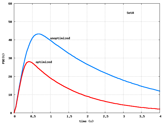
we could find for SetA and SetB are plotted in Fig.1, together with the

{PDE}^{*} (t)

generated by the initial (unoptimized) parameter values. Clearly, the optimization process has greatly improved the peak, and both sets approximate well the target values

TGTpk

TGTpktime

Fig.1a

Fig.1b

Figure 1: Step 3 optimization of SetA and SetB parameters:

{PDE}^{*} (t)

curves. Both sets approximate well the targeted peak (

TGTpk = 27

TGTpktime = 0.4

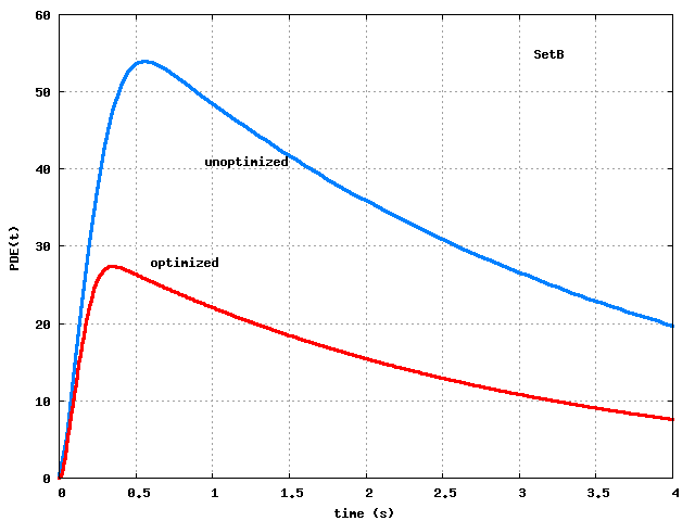
However, when we look at the resulting response curves, Fig.2, the peak-optimized parameters produce lousy overall response

R (t)

against the experimental data, even though they do well at the peak.

Fig.2 Figure 2: Step 3 optimization of SetA and SetB parameters:

R (t)

curves. Both sets do well at the peak but poorly afterwards.

Clearly, the strategy of optimizing to match only the peak is not sufficient.

4.4 Step 4. Optimization over the entire response history:

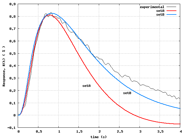
The failure of the peak-only optimization makes it necessary to optimize over the entire history of the data ! That's bad news, as there are too many data points (400, one every 10 msec), and the data curve (solid curve in Fig.2) is too wiggly. So, we first smoothed out the wiggly experimental data, and digitized the smoothed curve using only 32 time points, as shown in Fig.3.

Fig.3 Figure 3: Experimental data (wiggly curve), smoothed (dotted curve), and digitized using only 32 points.

These digitized points were used as $R_{tgt} (t_{k})$ points to minimize the L

^{2}

-norm of

R (t_{k}) - � � R_{tgt} (t_{k})

. In fact, we seek (influential) parameters

p_{1}, p_{2}, p_{3}, p_{4}

that mininize the multi-objective cost function

F (p) = \sum_{k = 1}^{32} {[1 - R (t_{k}) / R_{tgt} (t_{k})]}^{2} + w_{1} {[1 - R_{peak} / TGTpk]}^{2} + w_{2} {[1 - R_{pktime} / TGTpktime]}^{2}

(3)

with target values

TGTpk

TGTpktime

now set to those of the experimental response (0.82% and 0.7 sec, respectively), and various weights

w_{1}

w_{2}

. Note that the response values

R (t_{k})

k = 1, . . . 32

, as well as peak value,

R_{peak}

, and the time it occurs,

R_{pktime}

, are functions of the parameters

p

, in particular of

p_{1}, p_{2}, p_{3}, p_{4}

over which we are optimizing, and they can only be found by running the cascade code.

The NEWUOA optimization code is efficient and typically uses fewer than 100 evaluations of the cost function

F (p)

, for tolerance set to 2 %.

The multi-objective cost function

F (p)

, natural as it is for the problem, is far from ideal, unfortunately. It turns out that many

p

can produce about the same value for

F (p)

, and the starting

p

is crucial, a nightmare for optimization. Apparently, the landscape of

F (p)

is extremely "bumpy", with multiple, shallow, local minima. Moreover, it is very hard to drive

R_{pktime}

lower (desirable), and the last two terms in

F (p)

seem to antagonize each other; parameters that would lower

R_{pktime}

also drive

R_{peak}

away from the target value. Under the circumstances, the choice

w_{1} = 1

w_{2} = 5

for weights seems to do better than other combinations, yet leaves a lot to be desired.

As in the peak-only case of Step 3, there is high degree of non-uniqueness, and the values that minimize

F (p)

were usually not the best. So, again, we used the optimizer as landscape explorer, by printing out all the iterates to find (by inspection) those with best combination of

R_{peak} (p)

and

R_{pktime} (p)

, and then looking at the overall fit to the data.

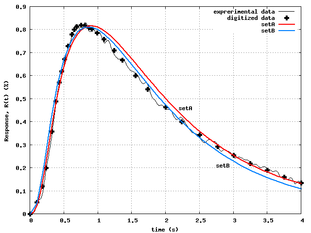
Fig.4 shows the best results we could obtain, after many tries with various combinations of weights, tolerances, and combinations of Step 3 and Step 4 optimizations. In fact, the SetA curve was obtained by Step 4 optimization applied to the Step 3 optimized SetA parameters, whereas the SetB curve was obtained directly by Step 4 optimization of the unoptimized SetB parameters. Considering the extreme natural variability of biological data, the agreement of both SetA and SetB response curves with the experimental data is very good.

Although both SetA and SetB do comparably well in capturing the data, their optimized parameters are quite different, exhibiting the severe non-uniqueness of the parameter estimation problem. For example, the

p_{1}, p_{2}, p_{3}, p_{4}

optimized values of SetA are 347 , 618 , 0.258 , 0.051, while those of SetB are 190 , 741 , 0.279 , 0.108. Viewed from another perspective, perhaps the values are not that different. A range of values for each parameter is perhaps the best one can hope to determine on the basis of indirect biological data.

Fig.4 Figure 4: Response from optimized SetA and SetB parameters, compared with the experimental data and the 32 digitized data points used in optimization.

5 CONCLUSION

We discussed parameter estimation by fitting to experimental data for phototransduction in rod photoreceptors of vertebrates. This is a typical inverse (ill-posed) problem of parameter identification that can be viewed as a multi-objective optimization problem. The difficulties encountered and procedures to overcome them were presented.

The difficulties include: large parameter space, highly nonlinear dependence of quantities of interest on the sought parameters, lack of good starting values, and high degree of non-uniqueness.

We employed statistical uncertainty and sensitivity analysis (using the excellent SimLab software package), to scope out the parameter space, to reduce the number of parameters to only the most influential ones, and to find "promising" starting parameter values for the subsequent multi-objective optimization problem. The ambiguities and pitfalls were pointed out. The fact that quantities of interest can only be found via simulation (running the forward model) necessitates using an efficient, derivative-free optimizer. Powell's NEWUOA fulfills these requirements.

Although natural for the problem, the multi-objective cost function

F (p)

is far from ideal. Its landscape seems to be extremely "bumpy", with multiple, shallow, local minima. Thus we resorted to using the optimizer as landscape explorer, by printing out the iterates to find (by inspection) those with best combination of

R_{peak} (p)

and

R_{pktime} (p)